A Physically Universal Cellular Automaton

Author’s note, November 2024: This post was originally published in June 2014 on my student website as an exposition of (Schaeffer, 2014). You can still see the original through the Wayback Machine, but I translated it to markdown and republished it here to get some practice with the new site generator. The text is unchanged, including references to ancient versions of Python and limitations of Golly which may or may not have been addressed at some point in the past decade. Also, don’t miss Scott Aaronson’s blog post about it! In fact, go read that first for some much-needed background on what we’re trying to do here.

This page is about an implementation of the cellular automaton from my physical universality paper (available here) in Golly, an open-source, cross-platform, cellular automaton simulator. We give a description of the cellular automaton and the construction in the paper, with more emphasis on the details of the implementation.

Files and Golly

You can find Golly here. The files below are for version 2.5 and up. You may also want to install Python to enable scripts in Golly. Python is not necessary for most basic operations in Golly, but we do use one script, goto.py, to jump ahead a large number of timesteps. Golly will look for Python 2.7 libraries, so install Python 2.7 and note that “a 32-bit version of Golly requires a 32-bit version of Python, and a 64-bit Golly requires a 64-bit Python”.

To see the CA and physical universality in action, all you need are these two files:

• PhysicColor.rule
• transformation.mc

The first file, PhysicColor.rule, tells Golly the states, neighbourhood, update rule, etc. for the cellular automaton. It should be placed either in your user rules folder (look under Preferences in Golly to see where this is) or in the Rules subfolder of your Golly installation. The second file, transformation.mc, is a pattern file, describing a specific configuration of the cells. All you need to do is open transformation.mc in Golly; it knows PhysicColor is the associated rule and will automatically use it (if it can find it). Note that transformations.mc is quite a large pattern, so you will need to zoom in (about 1000x) to see individual cells.

The Cellular Automaton

The CA is based on particles moving in two dimensions.

1. At discrete timesteps, each particle is at an integer point.
2. Each particle points in one of four directions: northeast, northwest, southeast, southwest.
3. There is at most one particle with a given position and direction.
4. Particles are indistinguishable.

The behaviour of the particles is defined as follows.

1. Each particle moves in the direction it points at a rate of one cell per timestep, until it meets other particles.
2. Particles interact where they meet, at integer or half-integer points.
3. When particles meet, they pass through each other unless there are exactly three particles.
4. When three particles meet, the two opposing particles reflect the third particle.

Implementation

Representation

Ideally we would represent the CA like this:

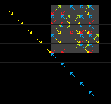
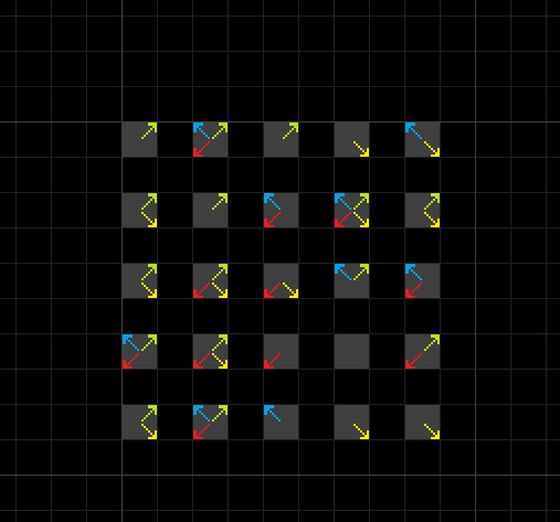
Each cell represents an integer point, and we draw arrows in the cell to represent the particles present at that point. We have colour-coded the particles by direction. Some of the cells are also marked gray, but this is purely cosmetic. We adopt this colour convention throughout: northeast (green), southwest (red), southeast (yellow), southwest (blue), with gray to mark regions.

Unfortunately, in this representation, the state of a cell depends on its current state (4 bits of information) and 12 bits from its neighbours. To implement the rule, we have to give Golly a table of all 65536 cases. To its credit, Golly happily accepts the massive rule table, but at some cost to performance. Instead, we will use a “sparse” representation, which looks like this.

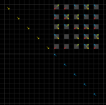
The particles are spaced out, with an extra row and column of empty space between them. We also split each timestep into two halves: the particles are at integer points in even timesteps, and at half-integer points in odd timesteps. Using the sparse representation, each cell depends on one particle from each of its four diagonal neighbours, so we can specify it with a table of only 16 rules.

In either case we use 16 states, whereas in the paper we only use two. The 16 state CA is still physically universal, but we would prefer a binary CA. The problem is that Golly is designed for Moore neighbourhood rules (especially Conway’s Game of Life) and has only limited support for Margolus neighbourhoods. It can simulate a given Margolus rule with a custom 5-state Moore neighbourhood rule, but the pattern has to be formatted like this:

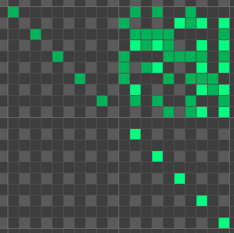
There are Python scripts available to convert patterns between this format and a truly binary representation, but they are unbearably slow on patterns of the size we are interested in. Since our CA maps empty space to empty space, we can construct a 5-state Moore CA where only live cells must be formatted.

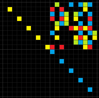
Overall, the advantages of simulated-Margolus representations do not outweigh their disadvantages, so we use the 16-state sparse representation discussed earlier.

Interactions

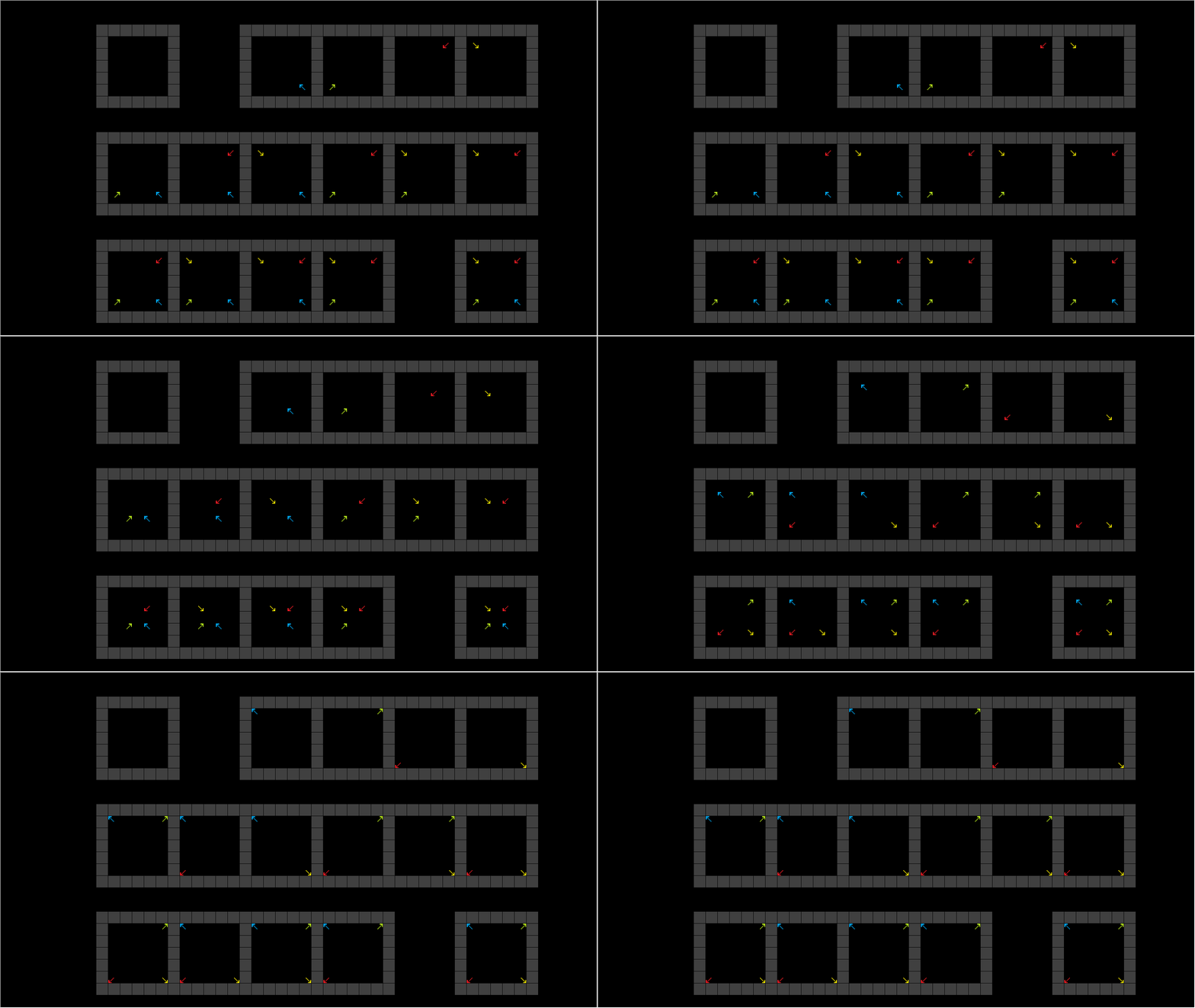
The interactions between particles are summarized in this table (including trivial zero- and one-particle interactions). Recall that particles only interact if there are exactly three particles present.

Physical Universality

A cellular automaton is physically universal if it can implement any transformation on any finite region by configuring the surrounding cells and letting the CA evolve. Let’s see an example in our CA. Open up file transformation.mc in Golly. You will be confronted with something like this:

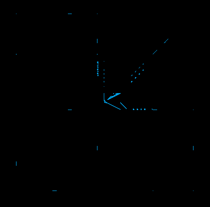
At this scale, all the particles appear blue because there are multiple cells per pixel, so blocks get represented by state 1’s colour (blue) if anything is alive, and state 0’s colour if everything is zero. Zoom in (say, by pressing ] thirteen times) to find the gray 5-by-5 square in the middle, at coordinates (0,0). The complex configuration around the gray cells is engineered to perform a transformation on the square if we let the CA run for 46754 timesteps. Golly provides the Python script goto.py to advance to a given generation quickly, or you use the regular controls and the generation counter at the top left.

After 46754 timesteps, the following pattern should replace the original gray square.

This is a transformation of our original input. If we go back to the beginning (Ctrl-R), change some of the gray cells, and step forward again, then the new output configuration will be the result of applying the transformation to the new input.

Physical Universality Construction

In this section, we will see how the configuration in file transformation.mc implements a transformation. There are three main steps:

1. Get the information out of the finite input region.
2. Perform the computation.
3. Fill the output region with the desired output.

Extracting the Input

We may assume the input region is a square, since any finite region is contained in a square region (i.e., bounding box) and we can extend the transformation from the region to the box arbitrarily. Extracting the input from the box is surprisingly simple:

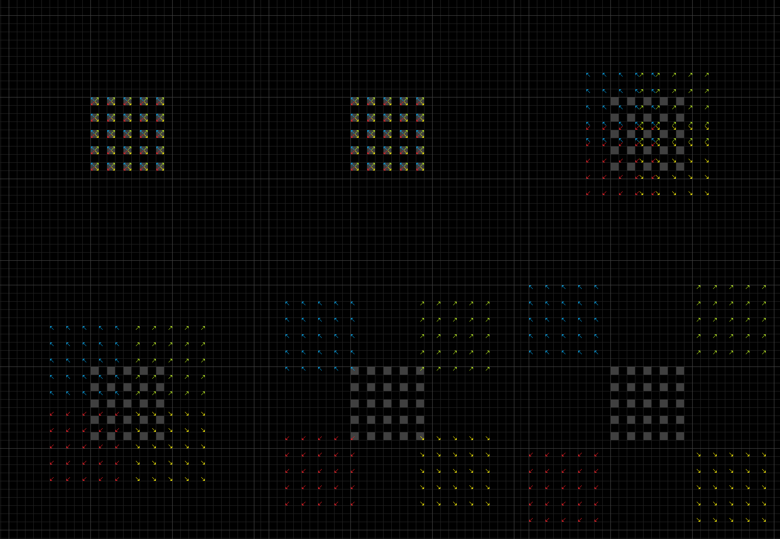
The particles literally escape on their own. Moreover, the particles exit the box quickly, and in orderly square groups. If some of the particles in the box are missing, then there will be holes in the groups.

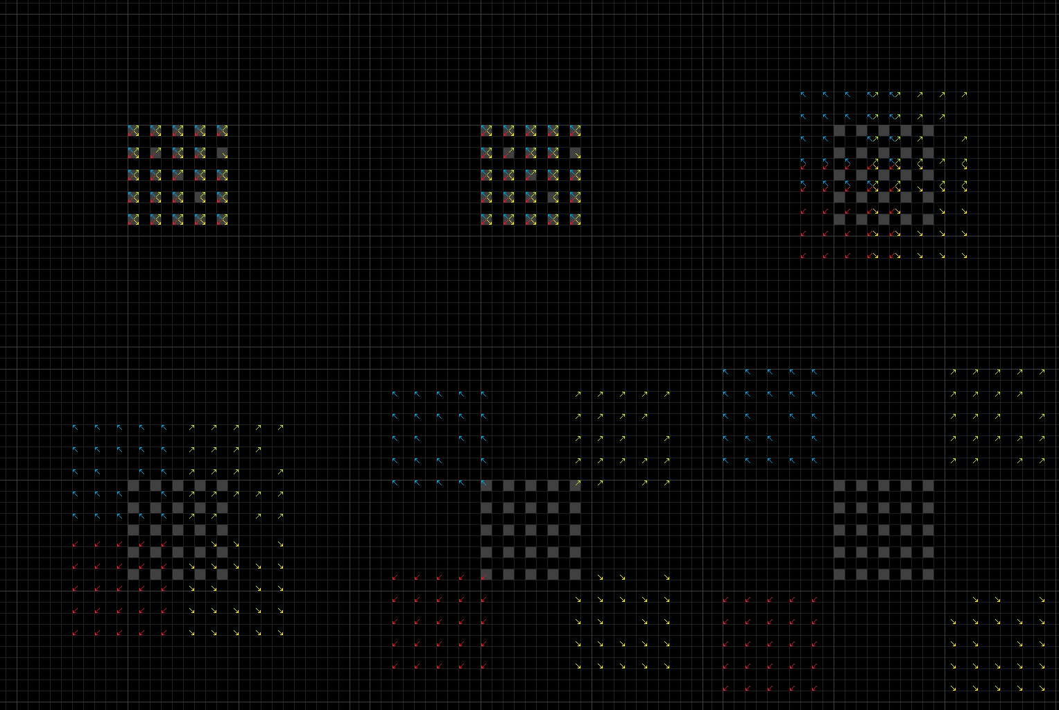
The presence or absence of particles in these groups tells us everything we need to know about the initial configuration of the box. We call these bits of information signals.

The computation phase will useall four groups to compute the output configuration. It is difficult to perform computations when the signals are moving in four different directions at the speed of light (i.e., as fast as they can move), so we will manipulate the signals into a column before we begin computation.

Redirecting the Input

Recall from the paper that we can reflect or deflect a signal. Suppose a signal is moving southeast. If we intercept it with two signals at right angles, then we have

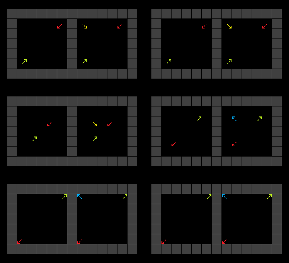
The signal leaves going northwest. On the other hand, if we intercept the signal with a particle in the opposite direction and a particle at right angles then we have this

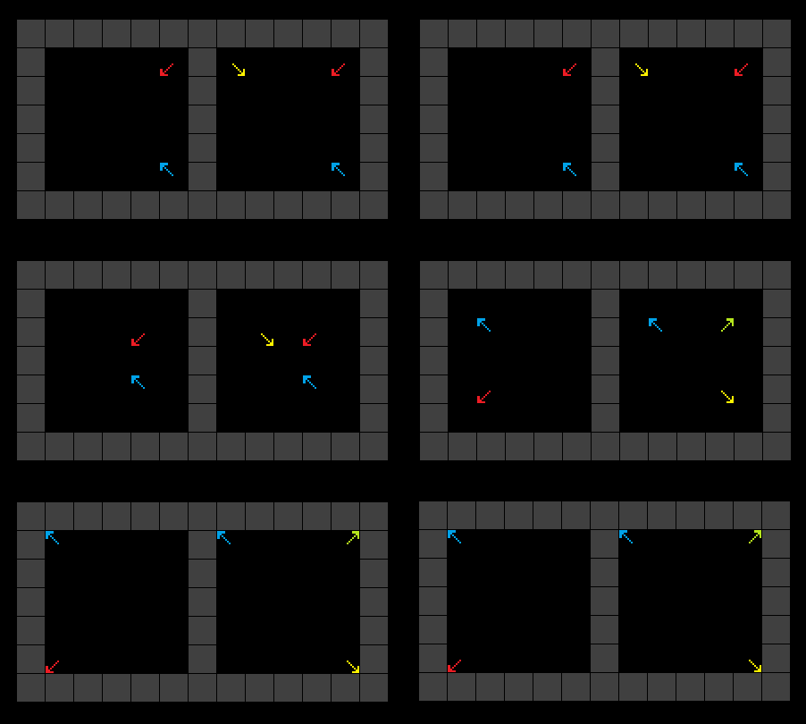
The signal continues through, but we get a copy of the signal (and its negation) at right angles.

With these two operations, we can essentially redirect particles however we like, given enough time. For example, at the very beginning we copy or rearrange signals so that all the information from the four square groups is moving northeast. See below.

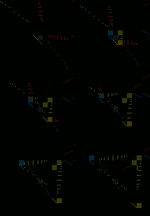
The short yellow and blue lines of particles (southwest of the box) reflect the southwest group before it can even leave the box. Meanwhile, the red blob to the east, and the blue curve below intercept the group moving southwest and deflect a copy of the information as a green blob. The same happens on the other side, so we end up with two blobs and two squares moving northeast, carrying all the information about the input with them. Next, we want to take the cloud of signals moving northeast and rearrange them into a column. This is done in two steps.

First, we rearrange the signals so there is at most one signal along each northeast/southwest diagonal. The two blobs already have one signal per diagonal, but the two square groups need to be fixed.

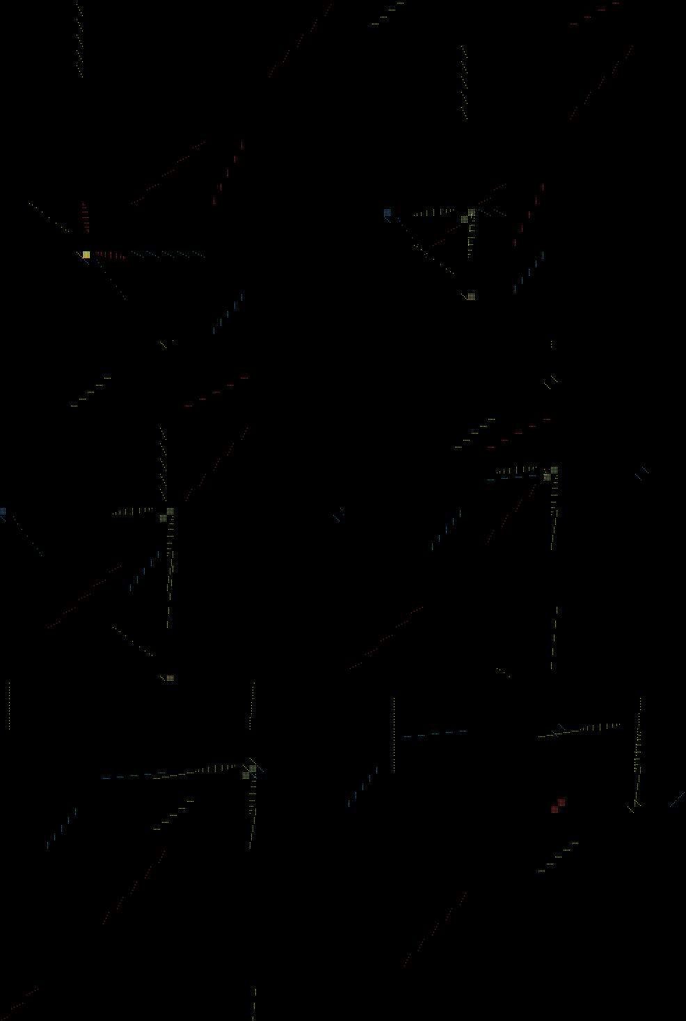
You can see five yellow pulses meet five red pulses and one of the square groups. This creates five blue pulses, moving west relative to the group, carrying all the information from that square group. Then another five yellow pulses and five red pulses fix the blue signals into five green lines, to the west of one of the green blobs. The same thing happens to the other square group. Once we have copied both groups, we no longer need them, so two pairs of yellow and blue lines reflect the groups southwest.

Second, we reflect each signal backwards for just the right amount of time to align all the signals into a column.

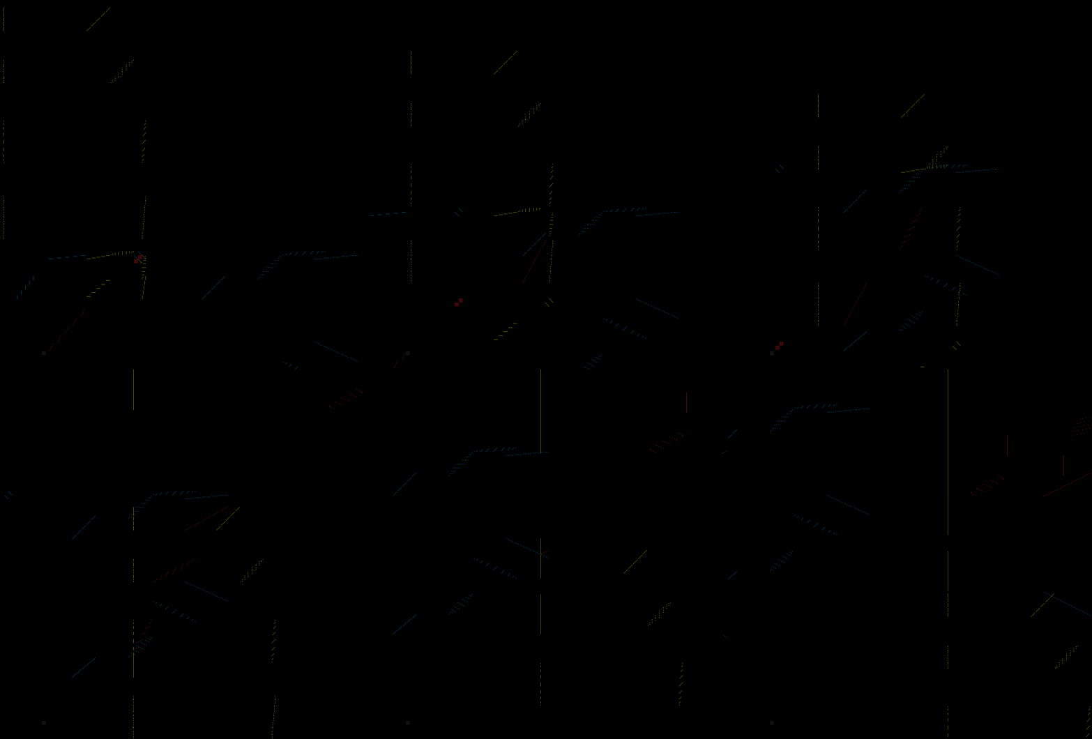
Here blue and yellow structures intercept the green signals, reflecting them backwards (in red), where another pair of blue and yellow structures align them into a column. Note that the second set of yellow structures are themselves in a column. In fact, the yellow particles are in the same column as the green signals, so it is unfortunately a bit difficult to distinguish one from the other.

Computation and Output

All computations are done using the interaction below. A red particle meets two unknown signals from the southwest and northwest.

Call the yellow signal x, and the green signal y. A particle escapes moving southeast if and only if x and not y.

In practice, the input signals, and signals for intermediate computations are in a column formation moving northeast. We implement a logical gate by sending a (yellow) particle, the runner, southeast through the column. The runner passes all of the signals along the way. We send red particles from the northeast to intercept the runner when it meets the signals corresponding to the inputs of the gate. If any of those input signals is 1 (i.e., a particle is present) then the runner is reflected. The runner gets through if and only if all the signals are zero. Finally, a (blue) particle from the southeast meets the runner and a (red) particle from the northeast. This creates a new signal because the red particle is reflected into position if and only if the runner is present.

You can see the computation in transformation.mc below. The input signals are barely visible as a pair of lines at the bottom left. A long line of yellow particles on the left serve as runners. The gates are specified by the large red triangle. The red particles at the bottom edge of the triangle, along with corresponding line of blue particles (mostly out of frame, to the south), create the new signals used within the computation, and eventually the output signals.

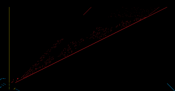
At this level of zoom, we can only see very high-level features of the transformation being implemented. You may be able to see a string of four to six parallelogram-like structures near the bottom of the red triangle, growing larger in the middle and smaller towards the ends. These implement circuits for decoding the original input configuration from the input signals, and then reencoding the output signals to achieve the desired output. This entails simulating the CA backwards on the 5-by-5 square for 5 steps. But if we watch the input diffuse out of the box in reverse, we see that when the four groups interact, it is initially only in a single cell, then 4 cells in the next step, 9 cells, and so on. There is a parallelogram for each step, but only the last two or three are large enough to be identifiable. Then the same thing happens in reverse for the output. The parallelograms are clearer when the input is larger.

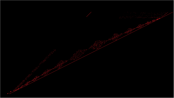
After the computation is complete, we reflect all the signals except the ones we want. Then a sequence of redirections puts the output signals into four square groups.

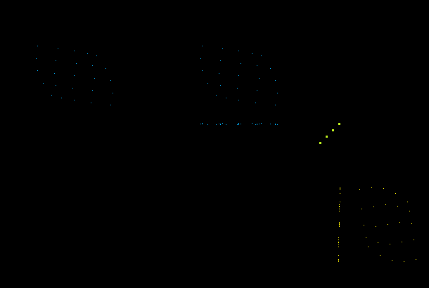
This only lasts for a moment (actually, a few thousand timesteps) before we redirect them again. Two of the groups will be reflected to arrive at the output at the desired time from the northeast and southwest. The other two groups are redirected to intercept two square configurations of particles, shown below.

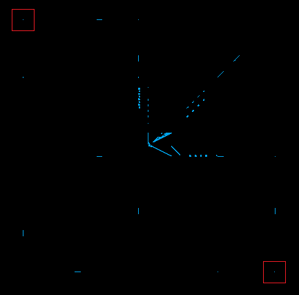
These two groups of particles were on a collision course from the very beginning, destined to meet in the gray box after 46754 timesteps. We carve out particles from these two groups to create the configurations we want. Eventually, the four groups converge on the gray square and produce the desired output.

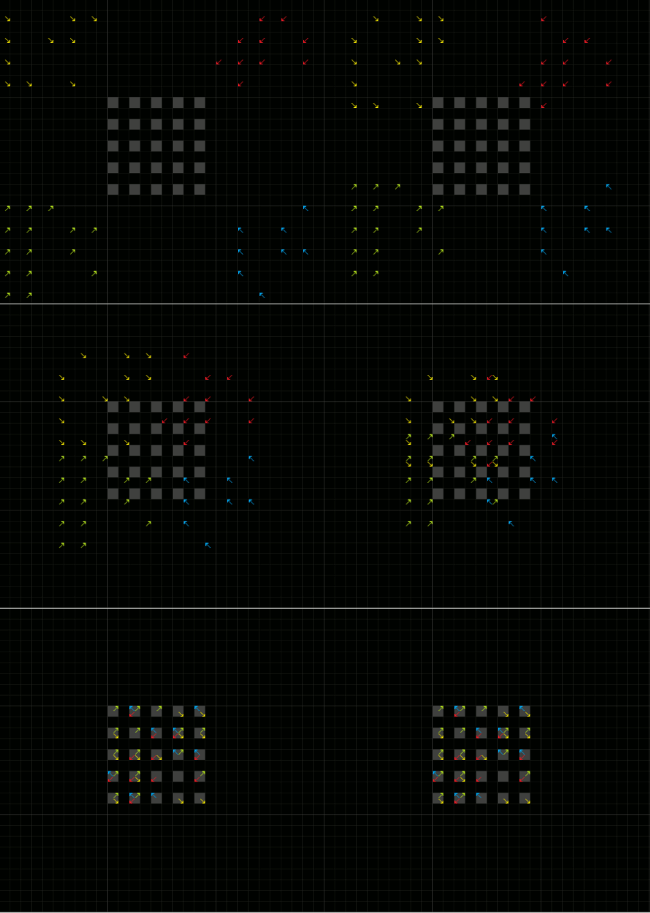
This completes the construction.